Introduction

This is our fifteenth Article and the third of five of a ‘mini-series’ on bond markets. In China, individual investors tend to prefer to invest in equities and real estate. But the bond market is a sector that we expect to grow in the coming years along with bond funds so that more individuals will invest in this sector. This third article of five, is intended to explain and illustrate the yield curve, which is the key model for trading and managing interest rate risk. The following Article 16 will look at how we trade bonds based on views of credit risk, the second major bond risk after interest rate risk:

16. Credit Risk and Corporate Bonds

17. Structured Securities

Present Value Calculations

In Article 11, we showed how to value a company using ‘discounted cash flow’ (DCF) method. The concepts of Present Value, Future Value, rates of return, are essential to finance. Bonds and money market instruments apply this concept of present value extensively. Just to review:

The price (value or present value) of a security is determined by forecasting what future cash flows will be earned, on what date and the appropriate rate of return/interest to discount them back to their current (present) value. Every bond and money market instrument is valued using that exact method. When teaching this in an academic program, tutors often simplify things to ‘whole years’ or ‘half years’, but we cannot do this in the real world.

Bond and money markets are based on ‘conventions’ or rules about how to calculate values of accrued interest. There will be ‘day-count conventions’ that stipulate the actual way you will calculate interest and, thus, price and your investment return. In every market I know about, we have a daily settlement convention. Thus, if you buy or sell at 10.53 on a Tuesday, you will calculate the accrued interest in exactly the same way as if you had sold it at 14.12 on that same day. China uses this same-day settlement convention as well.

In Article 14, we mentioned that it was a common convention to refer to a bonds yield-to-maturity (YTM). But, we also highlighted that was a bit simplistic and if we are going to manage bond portfolios we are going to have to use more precise definitions and analytics. We will take this journey in three steps:

1. We will describe and discuss the yield curve (sometimes referred to as the term-structure-ofinterest-rates) so that the reader understands the ‘real interest rates’ that apply in the market
2. From observed bonds on the yield curve (like government benchmark bonds) we will extract the zero-coupon yield for maturities from one-year to thirty-years
3. We will then illustrate a bond’s ‘duration’ to properly measure its price changes to any change in interest rates along the curve

If you can understand and master these three stages, then you are ready to invest in and/or trade interest-rate sensitive securities, like CGBs. Teaching these concepts at the university, we would go through a large number of algebraic proofs to derive all these individual values (zero-rates, duration, etc.). Though I will illustrate each on simply, I will show how you can get the relevant information from the various technology platforms that are used today.

The Yield Curve

The yield curve plots time-to-maturity on the (horizontal) X-axis and rates of interest on the (vertical) y-axis.

We can see, in general, the longer the investment horizon, the higher the rate of interest; we say the yield curve is ‘upward sloping’. This is normally the shape it is in all financial markets.

There are a great many factors, economic, financial and regulatory, that shape the slope and curvature of the yield curve. We will give a brief overview on two important drivers.

Central Bank Policy

The People’s Bank of China (PBoC) is tasked, among other things, to keep financial markets stable and to increase or reduce credit given its policy objectives. It may have administrative measures like key lending rates to commercial banks and it can also change the reserve ratios of deposits commercial banks leave with the PBoC. But, the main measure of influencing monetary conditions is through ‘open market operations’ (OMO). Here the PBoC sells financial securities (like CGB’s) to banks and thus takes money out of the financial system. To increase cash in system (ease credit conditions) it would buy financial securities from commercial banks.

As OMO tend to be very short-term in nature, one-day to maybe a year, this just affects the shortest rates directly, though the bank hopes it also has indirect affects on longer terms rates. People who trade in the bond market spend a lot of time analyzing the actions of the PBoC.

Economic Fundamentals

While the short end of the yield curve is very under the control of the PBoC, the long end is much more under the influence of long-term fixed income investors, and their analysis of macroeconomic trends, the nominal yields that they will accept in order to hold government bonds depend critically on what future inflation they anticipate. An increase in inflation expectations will mean bond investors require a higher rate of interest on any bond they are to buy.

Government Bonds and Pricing

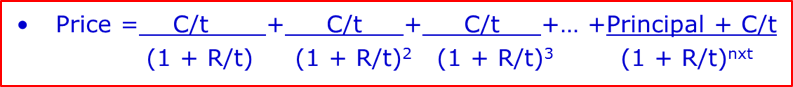
Revisiting our PV bond pricing formula below, we see that every cash flow has to be discounted back to the present by a single and unique rate of interest for that time.

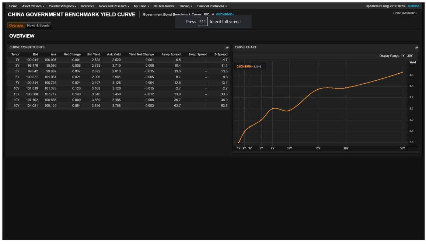
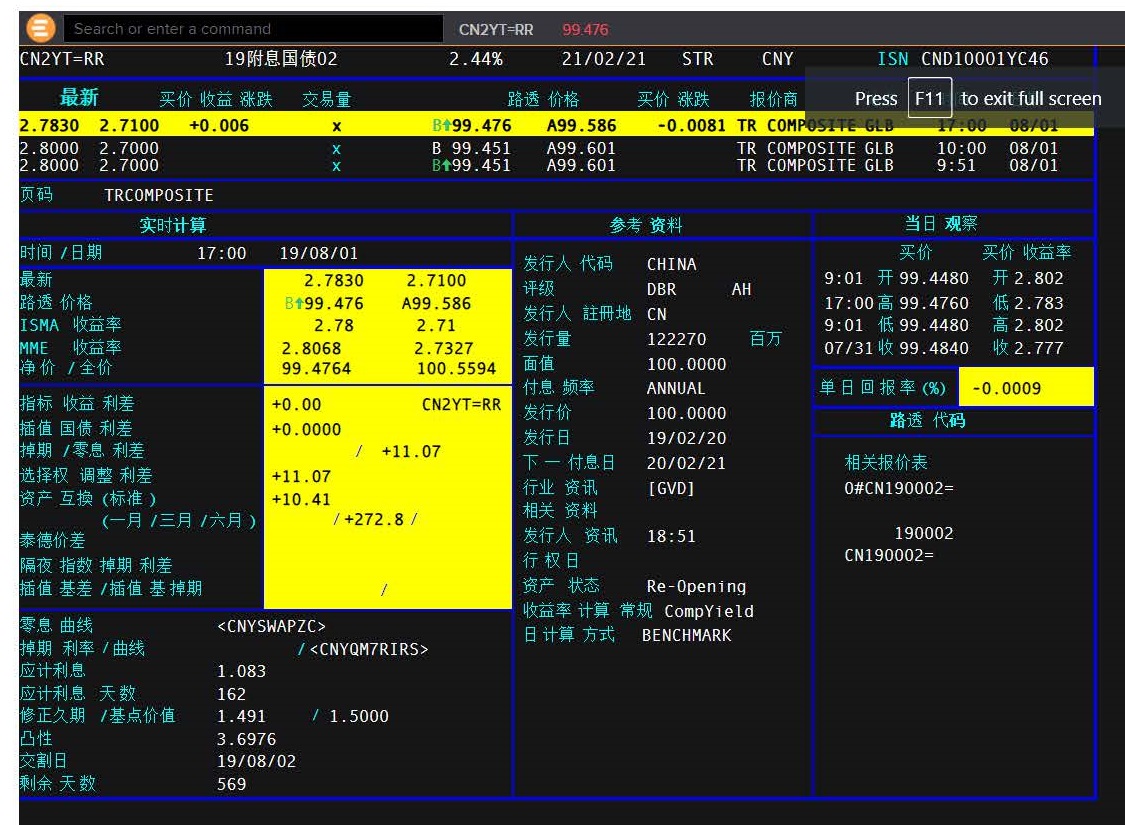
So, if you had a two-year investment that paid an annual coupon, you would need to discount the first annual payment at a unique rate for one year and the second payment (coupon and principal) at the two-year unique rate. But, we cannot just take a two-year government bond and use its YTM. Look at the CGB 2 year below where we see the YTM (bind) is 2.7830% (price 99.476). This is in effect a ‘blended rate’ of one (small) payment at one-year and one (larger) payment at two years. So, we cannot use this YTM to discount either the one-year payment or the two year. And we can see from our yield curve illustration above, the two-year rate is going to be higher than the one-year rate.

To do this, we go through an analytical process of ‘bootstrapping’ that allows us to extract the theoretical, unique rates for both one and two years. We refer to these as ‘zero-coupon’ rates as they reflect a unique interest rate, not part of a ‘bundle’ of payments in a coupon bearing bond. Deriving these zero-rates is rather complicated and won’t be illustrated here. Fortunately, any electronic terminal will generate these values for you.

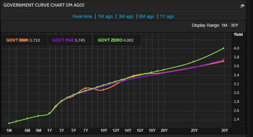
Benchmark (BMK) and Zero rates

We can see when the yield curve is upward-sloping (the normal case) that zero rates will be higher than the (blended) BMK YTM rates. This makes sense as the zero only reflects the longest period of the bond whereas the YTM average this long-rate with multiple shorter rates. (N.B. in the graph below I suspect the terminal took a ‘wrong rate’ around the 7-year maturity as it does not make sense that the YTM would be higher than the zero in this upward sloping market).

So, we have now illustrated our first two goals:

1. We will describe and discuss the yield curve (sometimes referred to as the term-structure-of-interest-rates) so that the reader understands the ‘real interest rates’ that apply in the market
2. From observed bonds on the yield curve (like government benchmark bonds) we will extract the zero-coupon yield for maturities from one-year to thirty-years

We have shown how by taking real bonds and rates (yield curve) we have extracted the theoretically correct zero-rates that are the basis for our valuation of any cash flow.

Bond Duration

Different bonds (even of the same issuer) have different characteristics, for example:

• CGB’s are issued with different coupons (note that 2-year coupon is 2.44% but the 5-year coupon is 3.19%)
• CGB’s are issued with different maturities (2, 5, 10, 30 and others)
• Market (discount) rates change with time

Measures of duration (be it Macaulay or Modified duration) are meant to create a single measure for each bond about its price sensitivity to a change in interest rates.

Looking at the 2-year bond illustration above, we see the Modified Duration is 1.491, less than its twoyear maturity. A bond’s duration (unless it is a zero-coupon bond) is always less than its term-tomaturity. Looking at the 5-year bond below, we see the Modified Duration is 4.332, again less than its five-year maturity.

We can rank bonds on their interest rate sensitivity by duration. The higher the duration, the more its price will change given a change in market interest rates. We can easily see that a 5-year bond is more sensitive to rate changes than a two-year bond. But, what if we had two 5-year bonds with different coupons? If they had the identical maturity date then the 5-year bond with the higher coupon would have a lower duration – and this be less at risk to change in interest rates. Duration can be a powerful tool to help you manage interest rate risk for many bonds with varying characteristics (term, coupon and varying levels of market interest rates).

Bond investing is a very quantitative subject, more so than equities. Much of the mathematical tools are now programed into computers and so you do not have to manually value bonds, calculate duration, etc. But, understanding these concepts gives you greater intuition of how bonds will change price in the market and sometimes we need to make quick decisions and don’t have the time to do a lot of analysis. Understanding the ‘fundamentals’ of valuation is always of importance.

In Conclusion

This article focused on the first key risk of bond markets, interest rate risk. For bonds with low perceived credit risk (like CGBs), it is interest rates that drive changes in a bonds value. We have demonstrated how to properly value these bonds using the term-structure-of-interest-rate or yield curve. This is a core topic in understanding and investing in bonds.

We will see in Article 16 that when a bond is issued by a very low rated entity, it sometimes takes on ‘equity-like’ characteristics. Thus, the topic of credit risk then also becomes important to these corporate bonds.

John D. Evans, CFA (author) has over 24 years’ experience in the international capital markets working with issuers of securities and investors around the world. He has designed and taught Master’s programmes in investment management at universities in the UK and China. He was most recently Professor of Investment Management at XJTLU in Suzhou. He now manages SEIML, a consultancy to early-stage companies in China.

Jina Zhu (translator) did her Master’s in Economics in France and is fluent in Mandarin, English and French. She also works at SEIML supporting early-stage companies grow and raise capital in China.

10 October 2019